Graph Convolutional Network Implementation With the PROTEINS Benchmark Dataset

This is part four in a series on graph theory and graph convolutional networks.

If you’ve been reading this whole series, you’ve been with me on this entire journey — through discussing what graph theory is and why it matters, what a graph convolutional network even is and how they work, and now we’re here, to the fun part — building our own GCN.

If you’re new to this series, that’s totally fine, too! In either case, let’s get coding!

For this tutorial, we’re going to be walking through two implementations of GCNs to classify the PROTEINS benchmark dataset. If you want to find attribution or papers on this data, or download it to look at it yourself, you can find it here under the “Bioinformatics” heading. You can also take a look at the whole notebook here. Attributions for the code can be found in the repository for this project.

If this in-depth educational content is useful for you, subscribe to our AI research mailing list to be alerted when we release new material.

Part I: GCNs with Spektral

What is Spektral? According to their homepage:

Spektral is a Python library for graph deep learning, based on the Keras API and TensorFlow 2. The main goal of this project is to provide a simple but flexible framework for creating graph neural networks (GNNs).

Getting started with Spektral is extremely easy because of the forethought put into the project — if you’ve done any modeling with Keras or Tensorflow, I think you’ll find Spektral quite intuitive.

Additionally, Spektral has many benchmark graph datasets built in, meaning that you avoid the fuss of needing to ensure your data is in the right format for modeling with GNNs, and can easily get started experimenting.

Whether you’re following this tutorial in Colab or just a plain ol’ Jupyter Notebook, our first step will be the same. Spektral is not one of the built-in libraries in Colab, so we’ll need to install it:

!pip install spektral

PROTEINS is one of the benchmark datasets for graph kernals from TU Dortmund. You can access this class of datasets from the TUDataset class, which we access by first importing and then instantiating an object of it, with the name of which TUDataset we’d like to access passed in:

1
2
3
4
5
6
# Reading in the PROTEINS dataset
from spektral.datasets import TUDataset
 
# Spectral provides the TUDataset class, which contains benchmark datasets for graph classification
data = TUDataset('PROTEINS')
data

When we load in our dataset, we can see how many graphs it contains in the n_graphs property. Here, we can see that this dataset has 1113 graphs. In this dataset, these are split into two distinct classes.

Spektral’s GCNConv layer is based off of the paper: “Semi-Supervised Classification with Graph Convolutional Networks” by Thomas N. Kipf and Max Welling. This is perfect, as this is the paper we’ve been referencing if you’ve been following this series so far. If you haven’t, I’d recommend checking out the paper as well as my article on how these networks work to get a better grasp on what Spektral is doing for us behind the scenes!

Since this is the layer we want to use, we’re going to have to perform some preprocessing. Spektral makes this super easy with their GCNFilter class, which performs the preprocessing steps (outlined in the paper) for us in just two lines of code.

First, import GCNFilter from spektral.transforms , and then call .apply() on our dataset, passing in the instance of GCNFilter :

1
2
3
4
# Since we want to utilize the Spektral GCN layer, we want to follow the original paper for this method and perform some preprocessing:
from spektral.transforms import GCNFilter
 
data.apply(GCNFilter())

At this stage, we want to be sure to perform our train/test split. I do this by shuffling the data and then taking slices (about 80/20% respectively) for this simple example, but you’re welcome to optimize this step further once you get comfortable with this implementation!

1
2
3
4
5
6
# Split our train and test data. This just splits based on the first 80%/second 20% which isn't entirely ideal, so we'll shuffle the data first.
import numpy as np
 
np.random.shuffle(data)
split = int(0.8 * len(data))
data_train, data_test = data[:split], data[split:]

Now, let’s import the layers we’ll need for our model:

1
2
3
4
5
6
7
# Spektral is built on top of Keras, so we can use the Keras functional API to build a model that first embeds,
# then sums the nodes together (global pooling), then classifies the result with a dense softmax layer
 
# First, let's import the necessary layers:
from tensorflow.keras.models import Model
from tensorflow.keras.layers import Dense, Dropout
from spektral.layers import GCNConv, GlobalSumPool

Wait a minute — aren’t these import statements from Keras? Don’t worry — this isn’t by accident. Because Spektral is built on top of Keras, we can easily use the Keras functional API to build our model, adding in Spektral specific layers as we go to handle the graph-structured data.

We import Dense and Dropout layers — Dense is your typical dense neural network layer that performs forward propagation, and Dropout randomly sets input units to 0 at a rate which we set. The intuition here is that this step can help avoid overfitting*.

Then, we import our GCNConv layer, which we introduced earlier, and our GlobalSumPool layer. Spektral defines this layer concisely for us:

A global sum pooling layer. Pools a graph by computing the sum of its node features.

And that’s all there is to it! Let’s build our model:

1
2
3
4
5
6
7
8
9
10
11
12
13
14
15
16
17
18
19
20
21
22
23
# Now, we can use model subclassing to define our model:
 
class ProteinsGNN(Model):
 
  def __init__(self, n_hidden, n_labels):
    super().__init__()
    # Define our GCN layer with our n_hidden layers
    self.graph_conv = GCNConv(n_hidden)
    # Define our global pooling layer
    self.pool = GlobalSumPool()
    # Define our dropout layer, initialize dropout freq. to .5 (50%)
    self.dropout = Dropout(0.5)
    # Define our Dense layer, with softmax activation function
    self.dense = Dense(n_labels, 'softmax')
 
# Define class method to call model on input
  def call(self, inputs):
    out = self.graph_conv(inputs)
    out = self.dropout(out)
    out = self.pool(out)
    out = self.dense(out)
 
    return out

Here, we use model subclassing to define our model. We’re going to pass n_hidden : the number of hidden layers and n_labels : the number of labels (target classes) to our model when we instantiate it for training.

Then, within __init__ , we define all of our layers as properties. Within call , we define this method to create and return our desired output by calling our layers on input in sequence.

Let’s instantiate our model for training!

1
2
# Instantiate our model for training
model = ProteinsGNN(32, data.n_labels)

Here, we’re going to initialize 32 hidden layers and the number of labels our data have. Spektral conveniently gives us an n_labels property on our TUDataset when we read it in. The benefit of this is that you can use this same code with any other Spektral dataset without modifications if you’d like to explore other data!

1
2
# Compile model with our optimizer (adam) and loss function
model.compile('adam', 'categorical_crossentropy')

Above, we’re calling .compile() on our model. If you’re familiar with Keras, you’ll be familiar with this method. We’ll pass in our optimizer, adam , and define our loss function, categorical crossentropy .

Now we reach a snag. Those of you familiar with Tensorflow and Keras might be tempted to just try to call model.fit() and call it a day. However, even though Spektral makes the process of building GNNs seamless on top of Keras, we can’t exactly work with our data the same way.

Because we’re using graph-structured data, we need to create batches to feed our Keras model. For this task, Spektral still makes our lives easier by providing Loaders.

1
2
3
4
5
6
7
8
# Here's the trick - we can't just call Keras' fit() method on this model.
# Instead, we have to use Loaders, which Spektral walks us through. Loaders create mini-batches by iterating over the graph
# Since we're using Spektral for an experiment, for our first trial we'll use the recommended loader in the getting started tutorial
 
# TODO: read up on modes and try other loaders later
from spektral.data import BatchLoader
 
loader = BatchLoader(data_train, batch_size=32)

Now that we’ve taken care of batching, we can call model.fit() . We won’t need to specify batches, just pass in our loader, since it works as a generator. We will need to provide our steps_per_epoch parameter for training.

1
2
3
4
# Now we can train! We don't need to specify a batch size, since our loader is basically a generator
# But we do need to specify the steps_per_epoch parameter
 
model.fit(loader.load(), steps_per_epoch=loader.steps_per_epoch, epochs=10)

For this simple example, we’ve only chosen 10 epochs. To validate, let’s create a loader for our test data:

1
2
3
# To evaluate, let's instantiate another loader to test
 
test_loader = BatchLoader(data_test, batch_size=32)

And we’ll feed it to our model by calling .load() .

1
2
3
4
5
# And feed it to our model by calling .load()
 
loss = model.evaluate(loader.load(), steps=loader.steps_per_epoch)
 
print('Test loss: {}'.format(loss))

That concludes building GCNs with Spektral! I urge you to play around with optimizing this example, or diving into other GNNs you can build with Spektral.

Part II: GCNs with Pytorch-Geometric

Even though Spektral gives us an excellent library of graph neural network layers, loaders, datasets, and more, there are times where we might want a little more fine-tuned control, or where we might want to have another tool for the job.

Pytorch-Geometric also provides GCN layers based on the Kipf & Welling paper, as well as the benchmark TUDatasets. Implementation looks slightly different with PyTorch, but it’s still easy to use and understand.

Let’s get started! We’ll be working off of the same notebook, beginning right below the heading that says “Pytorch Geometric GCN”. Attribution for this code is provided.

Our first step, as usual, is to install our required packages:

# Install required packages.
!pip install -q torch-scatter -f https://pytorch-geometric.com/whl/torch-1.8.0+cu101.html
!pip install -q torch-sparse -f https://pytorch-geometric.com/whl/torch-1.8.0+cu101.html
!pip install -q torch-geometric

Now, let’s grab our dataset:

1
2
3
4
5
import torch
from torch_geometric.datasets import TUDataset
 
# Like Spektral, pytorch geometric provides us with benchmark TUDatasets
dataset = TUDataset(root='data/TUDataset', name='PROTEINS')

And take a look into our data:

1
2
3
4
5
6
7
8
9
10
11
12
13
14
15
16
17
18
19
20
21
# Let's take a look at our data. We'll look at dataset (all data) and data (our first graph):
 
data = dataset[0]  # Get the first graph object.
 
print()
print(f'Dataset: {dataset}:')
print('====================')
# How many graphs?
print(f'Number of graphs: {len(dataset)}')
# How many features?
print(f'Number of features: {dataset.num_features}')
# Now, in our first graph, how many edges?
print(f'Number of edges: {data.num_edges}')
# Average node degree?
print(f'Average node degree: {data.num_edges / data.num_nodes:.2f}')
# Do we have isolated nodes?
print(f'Contains isolated nodes: {data.contains_isolated_nodes()}')
# Do we contain self-loops?
print(f'Contains self-loops: {data.contains_self_loops()}')
# Is this an undirected graph?
print(f'Is undirected: {data.is_undirected()}')

Here, it’s demonstrated that there are a variety of properties provided by Pytorch-Geometric on our TUDataset object. This provides us a lot of information that we can use to fine-tune our approach later, as well as deeply understand our data.

Now that we know what our data looks like, we’re going to perform our train/test split. For this example I also use a simple shuffling and then slicing method, but as always, I encourage you to look into optimizations for this step!

1
2
3
4
5
6
7
8
9
10
11
12
# Now, we need to perform our train/test split.
# We create a seed, and then shuffle our data
torch.manual_seed(12345)
dataset = dataset.shuffle()
 
# Once it's shuffled, we slice the data to split
train_dataset = dataset[150:-150]
test_dataset = dataset[0:150]
 
# Take a look at the training versus test graphs
print(f'Number of training graphs: {len(train_dataset)}')
print(f'Number of test graphs: {len(test_dataset)}')

Pytorch also provides us with DataLoaders for batching:

1
2
3
4
5
6
7
8
# Import DataLoader for batching
from torch_geometric.data import DataLoader
 
# our DataLoader creates diagonal adjacency matrices, and concatenates features
# and target matrices in the node dimension. This allows differing numbers of nodes and edges 
# over examples in one batch. (from pytorch geometric docs)
train_loader = DataLoader(train_dataset, batch_size=64, shuffle=True)
test_loader = DataLoader(test_dataset, batch_size=64, shuffle=False)

Now that we’ve taken care of that step, we can build our model. We’ll use a similar approach, but remember that now we’re using Pytorch instead of Keras.

We’ll import our functional layer (similar to Keras’ Dense layer), our GCNConv layer, and a global_mean_pool layer. This performs a similar pooling operation as Spektral’s GlobalSumPool , but by taking the mean rather than the sum of neighboring nodes.

1
2
3
4
5
6
7
8
9
10
11
12
13
14
15
16
17
18
19
20
21
22
23
24
25
26
27
28
29
30
31
32
33
34
35
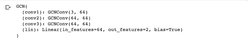
# Import everything we need to build our network:
from torch.nn import Linear
import torch.nn.functional as F
from torch_geometric.nn import GCNConv
from torch_geometric.nn import global_mean_pool
 
# Define our GCN class as a pytorch Module
class GCN(torch.nn.Module):
    def __init__(self, hidden_channels):
        super(GCN, self).__init__()
        # We inherit from pytorch geometric's GCN class, and we initialize three layers
        self.conv1 = GCNConv(dataset.num_node_features, hidden_channels)
        self.conv2 = GCNConv(hidden_channels, hidden_channels)
        self.conv3 = GCNConv(hidden_channels, hidden_channels)
        # Our final linear layer will define our output
        self.lin = Linear(hidden_channels, dataset.num_classes)
        
    def forward(self, x, edge_index, batch):
      # 1. Obtain node embeddings 
      x = self.conv1(x, edge_index)
      x = x.relu()
      x = self.conv2(x, edge_index)
      x = x.relu()
      x = self.conv3(x, edge_index)   
 
      # 2. Readout layer
      x = global_mean_pool(x, batch)  # [batch_size, hidden_channels]
 
      # 3. Apply a final classifier
      x = F.dropout(x, p=0.5, training=self.training)
      x = self.lin(x)
      return x
    
model = GCN(hidden_channels=64)
print(model)

When we build our model, we inherit from Pytorch’s GCN model, and then initialize three convolutional layers. We’ll pass in the number of hidden channels when we instantiate our model.

Then, we build a forward() method, which is similar to the call() method we build earlier in our Spektral GCN. This tells our model how to propagate our inputs through out convolutional layers. With Pytorch, we explicitly define our activation function. In this example, we use relu .

Prior to our final classification, we perform our pooling, and then set our dropout and pass our inputs through a final linear layer.

While there are a lot of opportunities to customize and fine-tune our Spektral model, I like how explicitly we define our architecture with Pytorch. When it comes to “which approach is better”, like most things, it depends on what your team needs to prioritize (explain-ability over efficiency of quickly proving concept, for example).

Let’s take a look at the resulting architecture:

Next, we’ll need to:

1. Set our optimizer — we’ll be using adam for this implementation as well
2. Define our loss function — similarly, we’ll keep categorical crossentropy
3. Define train and test functions, and then call them for a set amount of epochs.

1
2
3
4
5
6
7
8
9
10
11
12
13
14
15
16
17
18
19
20
21
22
23
24
25
26
27
28
29
30
31
32
33
34
# Set our optimizer (adam)
optimizer = torch.optim.Adam(model.parameters(), lr=0.01)
# Define our loss function
criterion = torch.nn.CrossEntropyLoss()
 
# Initialize our train function
def train():
    model.train()
 
    for data in train_loader:  # Iterate in batches over the training dataset.
      out = model(data.x, data.edge_index, data.batch)  # Perform a single forward pass.
      loss = criterion(out, data.y)  # Compute the loss.
      loss.backward()  # Derive gradients.
      optimizer.step()  # Update parameters based on gradients.
      optimizer.zero_grad()  # Clear gradients.
 
# Define our test function
def test(loader):
  model.eval()
 
  correct = 0
  for data in loader:  # Iterate in batches over the training/test dataset.
      out = model(data.x, data.edge_index, data.batch)  
      pred = out.argmax(dim=1)  # Use the class with highest probability.
      correct += int((pred == data.y).sum())  # Check against ground-truth labels.
  return correct / len(loader.dataset)  # Derive ratio of correct predictions.
 
  
# Run for 200 epochs (range is exclusive in the upper bound)
for epoch in range(1, 201):
    train()
    train_acc = test(train_loader)
    test_acc = test(test_loader)
    print(f'Epoch: {epoch:03d}, Train Acc: {train_acc:.4f}, Test Acc: {test_acc:.4f}')

We’re using many more epochs for this example, and as such, we achieve better metrics. There isn’t an inherent reason for this aside from the code examples I used to help build the models and learn each respective library. Also, given that the Pytorch-Geometric implementation was my final implementation, I focused more on results than in my earlier experiments. As always, I encourage you to play with and optimize the code and make it better!

Looking at the last 20 training epochs, we see that we achieve about 71.34% training accuracy and about 62.67% test accuracy. Evaluating accuracy on the test data around epoch 186, one potential optimization would be early stopping callbacks that ensure we stop training once we achieve convergence, to avoid overfitting the model.

There are more optimizations we can make, but this has been a long article, so we’ll stop here, and I’ll leave you to your own experimentation and optimization!

Notes:

* — For more information on dropout or why it works, check out this source.

This article was originally published on Towards Data Science and re-published to TOPBOTS with permission from the author.

Enjoy this article? Sign up for more AI updates.

We’ll let you know when we release more technical education.