How Can You Tell If Your Recommender System Is Any Good?

It’s an exciting time to be working on recommender systems. Not only are they more relevant than ever before, with Facebook recently investing in a 12 trillion parameter model and Amazon estimating that 35% of their purchases come from recommendations, but there is a wealth of powerful, cutting edge techniques with code available for anyone to try.

So the tools are at hand to build something neat to deliver personalized recommendations to your users! The problem is, knowing if it’s any good.

When John Harrison was developing the marine chronometer, which revolutionized long-distance sea travel by allowing ships to accurately determine their longitude, he had a problem with evaluation: to measure the device’s accuracy in practice required a long sea voyage. Similarly, the gold standard for evaluating a recommender system is expensive and time consuming: an A/B test, in which real users selected at random see the new model, and their behavior is compared to users who saw the old model. In both cases if this was the only way to evaluate, it would be impossible to try out new ideas with agility, or to quickly iron out flaws.

Instead, it’s necessary to have a quick, cheap way to evaluate a model. In the case of Harrison, he always built two clocks, and measured how much they diverged at his work bench. That gave him a metric of precision, which in turn let him iterate quickly on his design and get to a very high level of performance before a single ship ever put to sea — and indeed the first test journey, from London to Lisbon in 1736, showed his invention to be a success. For recommender systems, the solution is offline evaluation, where historical data is used to estimate how a user might have reacted to a different set of recommendations placed in front of them at a certain point in time, by using the knowledge of what they really did react to later.

With good offline evaluation, when we make something great we’ll know it. Conversely, without good offline evaluation a whole team could follow the wrong course for weeks or months, entirely at sea.

For fun and learning, I am building a recommender system for Wikipedia editors (aka Wikipedians) to suggest what article they should edit next, called WikiRecs. I’m especially interested in the interplay of timing and sequence of actions to predict what someone will do next in an app or on a website. There are several cutting edge AI techniques I am exploring to fully use all those sources of information, but from my background in science I knew that the first priority is trustworthy measurements, in this case via offline evaluation.

Offline evaluation requires figuring out how to make a valid test set, what metrics to compute, and what baseline models to compare it to. I’ll give my tips for these below, focusing on what is practical for industry rather than the higher bar of academic publication, but first a bit about my dataset. Wikipedia doesn’t have star ratings or thumbs up/thumbs down, so this is inherently an implicit recommendation problem, where my signal of interest is the choice to edit an article. Based on a user’s history of edits, and any other information I can pull in, I want to build a picture of their interests, in particular their recent interests, and learn to rank a personalized list of articles.

If this in-depth educational content is useful for you, subscribe to our AI research mailing list to be alerted when we release new material.

Here’s an example of what my Wikipedia data looks like, for my Swiss friend who goes by Rama. He has over 45,000 edits to Wikipedia since 2004, and very specific interests, mostly French naval history and computer technology.

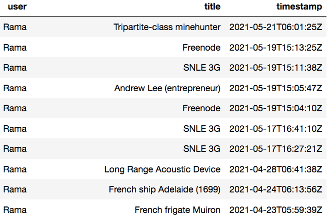
Using Wikipedia’s publicly available API, I sampled 1 million of the most recent edits for all users of English Wikipedia, which turned out to be only a few days worth of data. Then for each editor represented in the sample I pulled their last 1 year of edits, 21 million datapoints in total. Sampling like this only captures users who were active in this period — for one thing this will somewhat over-represent the most active editors, but that’s the population I am most interested in serving. I did some basic cleaning, e.g. removing bots and users with too many or too few edits, and then built my training set, test set, and baseline recommenders. The final training set covered 3 million Wikipedia pages (out of about 6.3 million total) and 32,000 users.

Here’s repo and notebook with all the code.

Tip #1: To craft your evaluation, first think about what the recommender system is for

There is no generic metric or evaluation procedure that will work for every use case. Every decision about the offline evaluation depends on what you are using the recommender system for.

Are you trying to DJ the ultimate 3 hour block of music for one person? Are you trying to get people to notice and click on a product in an ad? Are you trying to guess what a searcher wanted when they typed “green bank”? Are you trying to set a subscriber up with a date who’s a good match?

That will form the basis for answering questions like: What is the metric of success? How exactly do you separate out the test set? How far down the list can the relevant stuff be placed before it stops being useful? How important is resurfacing items they’ve already shown an interest in?

In my case, I envision WikiRecs as a sort of co-pilot for editing Wikipedia. A personalized list that you can glance at to give you ideas for the next article you might want to edit. I also want it to flexibly and continuously adjust to the user’s changing interests. Therefore I chose to focus my evaluation on how well the learn-to-rank algorithms predict the next page the user really edited. Formulating the problem in terms of short term prediction makes it an excellent candidate for sequential recommendation systems, in which the sequence and timing of the user’s actions is explicitly modeled.

Rather than predicting the next item, I could have taken a whole week or month of subsequent activity and predicted what was edited in that period, which would be a multilabel problem (and allow for additional metrics such as Precision@K), but this would require more data, add complexity, and shift the emphasis to more long-term predictions. I would take another approach again if my goal was to capture deeper, more permanent preferences of a user, that are expected to persist over the lifetime of their relationship with the app or tool.

A quick menu of articles to edit probably shouldn’t be more than about 20 items, so I chose metrics that rewarded putting the relevant items in the top 20. The first, basic metric to look at then is Recall@20 (also known as hit rate, in cases like this with only one relevant item): how often did this algorithm place the actual next article to edited in the top 20?

Tip #2: Be aware of model and position bias

When you are building a recommender system to replace an existing solution, there is a problem of position bias (AKA presentation bias): items recommended by the current system have typically been placed at the tops of lists, or otherwise more prominently in front of users. This gives those items an advantage in offline evaluation, since there will be a tendency to favor models that also place them at the top, regardless of how customers would react to them in practice. Therefore simple evaluation metrics will be conservative towards the existing system, and the improvement will have to be large to beat the “historical recommender” (the ranked list that was really shown to the customer).

There are a number of techniques for fighting this bias, in particular inverse propensity scoring, which tries to model the unfair advantage items get at the top and then downweight actions on them proportionally. Another approach, though costly, is to have a “holdout lane” in production where personalized recommendations were not served, and use that to at least provide evaluation data — it may not provide enough data to train on. The ultimate evaluation data might be truly random lists of items presented to some portion of users, but even if a company could afford the likely huge drop in performance, it probably wouldn’t want the trust busting (see below) experience that would give!

Luckily in my case I didn’t have to worry about position bias much. Editing a Wikipedia page is a pretty high-intent action, so there is little problem with people idly editing articles just because they’re in front of them. The edits have nothing to do with my recommender system (since it doesn’t exist yet), so I don’t have to worry about previous-model bias (a form of presentation bias). There could be popularity bias, with people rushing to edit the hot topic of the day, but as we’ll see below it’s not very strong.

Tip #3: Take care with picking the test set

For most recommendation algorithms, reliable evaluation requires a portion of the data to be set aside and used only for that. I have framed my recommendation problem as a forecasting problem, so I divided my data into the most recent action and everything that came before it. The baseline algorithms in this post (such as “most recently edited”), are all unsupervised, so they look at the historical data as the “training data” and the next action as the test data. However, when in the future I am evaluating algorithms that are supervised, I will also need to set aside a random sample of users, their history and most recent edit, from the same time range.

Takeaways: Make sure your training set doesn’t overlap your test set, and make two test sets, one being a dev set that can be used for tuning your hyper parameters rather than being used for the final evaluation.

Tip #4: Use a metric that considers position

Recall@20, how often the top 20 recs contain the next page that was edited, is a reasonable, blunt metric for comparing models for my task. However, learn-to-rank algorithms can be compared at a more fine-grained level by considering whether they put the relevant items closer to the top of the sort. This can be inspected visually by simply plotting Recall @ 1 through N, which can reveal positional differences.

For example, for a subset of the data (the “discovery set”, more on that later), the BM25 model has a higher Recall@20, but for the Recall@1, Alternating Least Squares scores better. Only by the 12th slot on the list is BM25 cumulatively better. That could indicate that BM25 is better at flagging relevant items, but ALS is better at making sure the most relevant appear at the top.

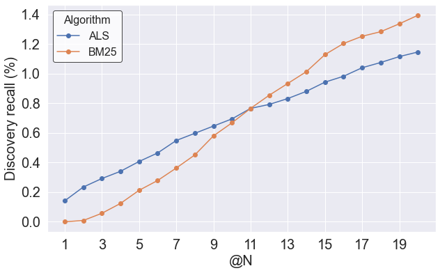
This positional performance can be boiled down to a single number using metrics such as MRR or nDCG that weight performance in the top positions more heavily. nDCG is a better choice in cases when there can be multiple relevant items to retrieve, and when those items might have different levels of relevance. But in my case, with a single relevant item in my test set, they are mathematically similar, equivalent to steep drop-off in “points awarded” as the algorithm places the relevant item further down the page. Reporting both would add nothing, so I arbitrarily decided to focus on nDCG@20, which has a score of 1 if the relevant item always appears in the first position, and 0 if it never appears in the top 20, and in between has an inverse-log drop-off of weighting by position. Sure enough, unfiltered ALS has a lower Recall@20 than BM25, but a higher nDCG@20.

Metrics such as Precision@K or MAP are not helpful in my case because of there only being a single relevant item. There are other metrics I didn’t compute that could be very helpful at distinguishing between algorithms, such diversity, coverage, and popularity bias.

Tip #5: Decide whether you care about discovery, resurfacing, or both

Many companies that rely on recommendations, such as Netflix or Amazon, make space in their interface for a special menu or carousel of recently visited items. Then their recommendation algorithms can focus on presenting users with items they’ve never interacted with, but might like: discovery. On the other hand, many recommendation systems just want to show users a list that contains personalized items that appeal, including resurfacing items they have already engaged with: discovery plus resurfacing. Examples of these kind of “single stream” recommendations include Spotify and YouTube play sequences, some e-commerce, and advertising.

Deciding what order to resurface items is a worthy challenge, with plenty of nuance, e.g. the role of time and how to decide whether a user has considered an item and rejected it. It is extremely relevant to e-commerce applications such as retargeting. But there are straightforward baselines for it: simply sort by recency of interaction or amount of interactions.

By contrast, getting good performance at discovery is a more open-ended question, with a real struggle to find a reasonable baseline. For one thing, even if a user has engaged with hundreds of items, there might be millions they haven’t.

But a challenge I’m really interested in is how to optimally combine discovery and resurfacing in a single list. Although past engagement with an item should carry lots of weight, if it was a long time ago or very out of character (I once clicked on a tacky carved wooden bed on Wayfair just to mess up my wife’s recommendations) a brand new recommendation that has high confidence should sometimes beat it.

For my Wikipedia recommendation task, I care about both discovery and resurfacing, and so my evaluation needs to reflect that. Many Wikipedians come back to the same articles over and over again, and my tool should make that convenient too, while mixing in new recs that it has high confidence that person would enjoy.

Therefore I split my test set into a discovery and resurfacing set, depending on whether the target most recent item had been edited by that user before, and computed all my metrics, including Recall@20 and nDCG, on both sets separately, as well as the combined test set.

By looking through raw edit histories, I noticed something that affected both my training and test set, which is that people often edit articles in bursts of two or more edits in a row. Often these are simply to correct a typo in the edit they just made. In my initial dataset I found that 35% of edits were to the previous page, so it’s far too easy to recommend the last edited article. It’s also not very useful, since that page is probably still open in one of that user’s tabs. So I changed my training set, and test set, to remove repeated edits in a block. I redefined my task, and my evaluation, to be: predict the next different article that is edited. This was a harder task, and my metrics fell accordingly. But it’s a task that more closely reflected what I mean when I think about recommendation quality.

After removing runs of edits, my training set was 30% resurfacing cases and 70% discovery cases. This mixture could affect the model’s predictions, so it might make sense to downsample or upsample to emphasize one or the other (it might also be worth trying training separate models on each set of cases). But the important part is to evaluate on them separately, to understand where the overall performance is coming from, and if it emphasizes one at the cost of the other.

Tip #6: Implement strong, simple baselines for comparison

“I built a deep learning recommender with 27 layers, 500 million trainable parameters, it’s wide, it’s deep, and it’s got inception, autoencoder and transformer components.”

“So how did it do?”

“Well it got a 0.4 nDCG.”

…Is that good? Even in the meticulous world of academic machine learning, there have been several high profile cases of innovative models failing to be compared to common-sense baselines, and when they are, failing to beat them — what has been called the “phantom progress” problem. Even if it’s not a new, experimental model type, failing to beat simple baselines is a good indication something has gone wrong with the implementation.

The only way to know for sure if you’ve made progress, and make sense of your metrics, is to implement some basic recommenders — the choice of which also depends on the problem.

I came up with three very basic ways to predict the next edited article:

• Popularity: Most popular over the past year
• Recent: Most recently edited by this user
• Frequent: Most frequently edited by this user in the last year

Then I implemented some slightly smarter, but still well understood collaborative filtering algorithms, which had mature, easy-to-use Python packages (specifically the Implicit package):

• BM25: Okapi BM25, a simple variation on Jaccard similarity with TF-IDF that often has much better results
• ALS: Alternating Least Squares matrix factorization of implicit training data, with BM25 pre-scaling

For these two I also computed “filtered” recommendations, with all the pages previously edited by that user removed, so recommending 20 items worth of pure discovery. These latter two used the same stripped-down training data: a user-item interaction count matrix (with 3 million by 32,000 entries, it was still very practical to load into RAM on my laptop thanks to SciPy sparse matrices!)

Another major benefit of implementing simple baselines is that it lets you kick the tires on every step of your data prep and model evaluation pipeline, essentially evaluating the evaluation. If the metrics for, say, Recent vs Popularity don’t make sense, much better to find it out at this stage rather than when trying to interpret results for a much more complex model. I found at least one massive bug in my evaluation this way!

Tip #7: Check for “trust busters”

Once I had my first set of recommender algorithms, I deliberately set aside time to look at the recommendations — to pore through the results and see how good they seemed intuitively, and get a qualitative idea of how the algorithms differed for individuals.

What I was looking for in particular were “trust busters” as the Netflix team called them, or “WTF@K” as another team calls them: recommendations for a user that come from so far out of left field that they seem like a glitch.

For Rama, only the Popularity recommender had obvious trust busting recommendations, with topics I happen to know he has no interest in, such as Zach Snyder’s Justice League. The ALS and BM25 algorithms leaned heavily on resurfacing, which makes sense for a 17 year veteran of the site. When new pages were forced (the “filtered” recs), they generally gave safe-looking selections of naval battles and French ships of the line. In the following table, resurfaced pages are bolded, and the correct next page in the dataset is colored red.

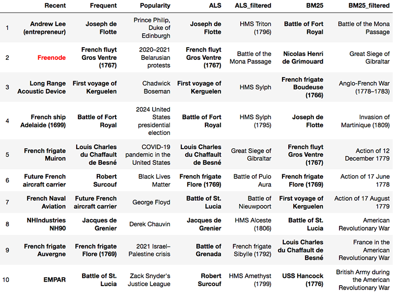
Interestingly, only the Recent recommender scored a hit in the top 10.

Besides Rama, I scrolled recommendations for a large number of other randomly selected users who had over 50 edits. It turns out that like my friend Rama, many Wikipedia editors have relatively small “beats” that they cover, and we should at least be able to nail recommendations for them. For example editor KingArti mostly cares about Marvel movies and TV series, and most of the algorithms picked up on that, though in different ways. Several also correctly predicted KingArti would edit Ms. Marvel (TV series) next. However, the top ALS recommendation is a fairly obscure 2003 Western series, Peacemaker, which might constitute a trust buster.

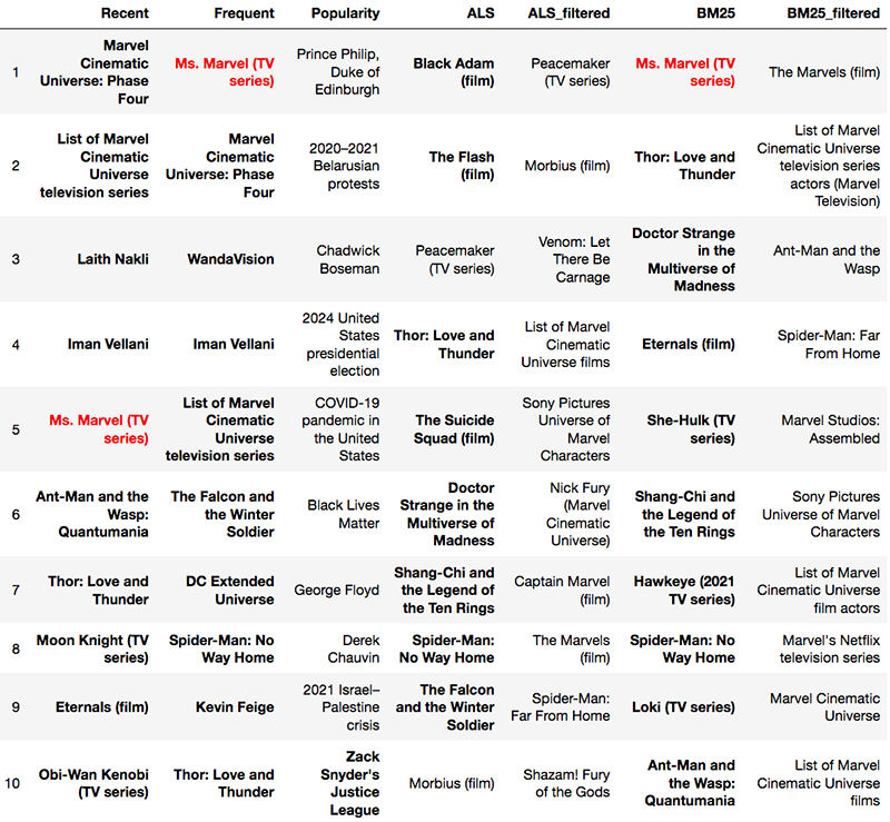
Among the observations I made is that BM25, when not filtered, has a bigger preference for resurfacing than ALS, which was later confirmed quantitatively.

Tip #8: Time spent optimizing your evaluation code is time well spent

At this point I’ll note that you are going to be running evaluation code over and over, more than you could ever have guessed, and the tighter you can make this loop, the quicker and more fun the process of finding your best model will be. Now is the time to leverage all the parallel compute you have available to you, whether it’s in the cloud or even just the multiple cores on your laptop, by using parallel computation tools like Spark, multiprocessing or joblib. There are packages, such as modin, that try to make simple Pandas parallelized transparently, so those might be good to check out.

I was lucky, but also purposeful, in choosing the Implicit library, because it is highly optimized and inherently parallel. Even still it took me embarrassingly long to realize there was a recommend_all function that was much faster than running recommend on each example. If you are using Scikit-learn, many operations have an n_jobs parameter — make sure to set that to -1 and it will be parallelized across all your cores.

Besides parallelization, it’s a good time to understand a bit better how things are computed behind the scenes, and invest in vectorization and refactoring heavy workloads that lean on Pandas, which is often incredibly slow. When I rewrote my recall curve function to use list comprehensions rather than DataFrame.iterrows(), it went from 2.5 minutes to 4 seconds per evaluation, and that made a huge difference.

Tip #9: Make sure your evaluation is reproducible

A horrible feeling is going back to recompute metrics and finding that what should be the same model on the same test set produces completely different scores. My two tips to prevent that (that I don’t always follow) would be:

• Check in your model code, evaluation code, and evaluation results at the same time so they match
• Rather than investing in a data versioning tool, follow this pattern and think of datasets as write-once, but then version control every step of the pipeline to clean and transform the data to produce your training and test sets.

Tip #10: Tune your baselines, but only to a point

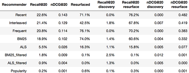
Not surprisingly, when it came to overall metrics Recent was hard to beat — people do tend to return over and over to edit the same pages. But the discovery test subset, where Recent was not useful, was much more interesting, and those recall and nDCG scores helped me distinguish among the collaborative filtering techniques.

It’s easy to come up with ideas for improving these baselines. For example, I could take Frequent algorithm and try limiting it to just the most frequent in the last 30 days, introducing a time element. For Recent I could only include recently edited items that were edited at least 5 times, or where the edit was above a certain size, e.g. 20 characters. But those are hand-tuned heuristics, which is exactly what we’re trying to get away from in ML projects. If you’re not in an academic setting trying to show incremental improvements, stop at something simple and easily explained.

Then there were the slightly less dumb baselines, which have tunable hyperparameters, but very few — BM25 and ALS had two, although I added BM25 scaling for implicit factorization, adding two more hyperparameters. But four is still a lot less than the number of hyper parameters for even the simplest neural network! I ran a couple of long grid searches to pick the final settings (K1 = 100, B = 0.25 for BM25), but didn’t worry too much about honing in on absolute perfection.

Surprisingly, the algorithm I was most hopeful about, implicit matrix factorization using ALS, didn’t perform the best at discovery. Instead the far simpler and faster BM25 approach beat it, both on the discovery set when filtered to just new items (by 240% on nDCG) and on the overall set when unfiltered. It’s still possible that I could find the right combination of hyperparameters, or even a different package, that would suddenly provide a breakthrough, but it’s just a baseline, and there are more powerful algorithms I’m itching to try.

Popularity did absolutely terribly — dead last on almost every metric, which matches the intuitions I had about this particular dataset from looking at specific examples. On Wikipedia people typically edit their own idiosyncratic interests, rather than chiming in on the issues of the day.

Tip #11: With good evaluation metrics, you can try solutions that are simple hacks— and that might be exactly what you want to ship

This may sound like a contradiction to tip #10 about not tinkering too much with the baselines, but it isn’t really!

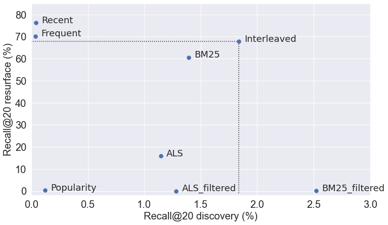
If I had to ship a Wikipedia recommendation algorithm this week, and it had to be good at both discovery and resurfacing, I might try simply interleaving the best resurfacing (Recent) and the best discovery algorithm (BM25 filtered), removing duplicates as I go. For my dataset I find that I get offline Recall@20 that is better than all other models except BM25 filtered at discovery, and only 11% worse than the best model at resurfacing. Furthermore, it clearly Pareto-dominates any of the other solutions that try to balance resurfacing and discovery.

It’s also seems clear to me from looking at Rama and KingArti’s Interleaved recommendations how it could be useful.

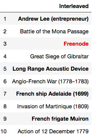
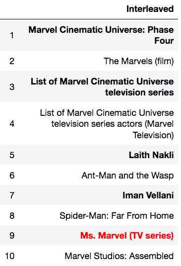
Sure, it’s a hack, but this interleaved output is a single-stream recommender that is simple to get right, produces highly explainable recs, and will run very fast in production. Something like this might be a great choice for a first system where there wasn’t personalization before — and until you’ve been through it, you won’t believe how many unexpected challenges there can be in productionizing even the simplest ML model, particularly if it needs to serve recs in realtime.

Tip #12: When possible, get qualitative feedback from users

Have you ever talked back to your Spotify Discover Weekly or your Netflix genre carousels? I have! I’ve noticed that I and my friends have intimate, opinionated relationships with the recommender systems in our lives. When the recs are good, but especially when they’re bad. We judge recs, we try to figure them out, and we even try to consciously shape them to be closer to what they want and expect. Ideally, you can make this kind of qualitative feedback part of your offline evaluation.

Many organizations don’t have a user experience department that you, as the modeler, have access to — though it’s worth checking! But even still, it might be a good idea to get informal feedback from friends and relatives who are already users, especially if you can show them different recommender outputs side by side. I sent Rama the output of these 7 baselines, and he wrote “a good balance between these extremes is struck by BM25_filtered” (between popular and articles familiar to him), also saying “the system is clearly finding subjects relevant to my interests and abilities.” Interestingly he also had memories of editing many of the pages in the filtered list, which means either he did but more than a year ago, or it’s just that good.

One final long-term thought: There are plenty of reasons why offline evaluation might not perfectly predict A/B test results, but if you are careful about it and compensate for some of the biases, hopefully it will at least predict the direction of results: the model that looks like a winner offline is a winner online. However, if you keep conscientious records over the course of multiple A/B tests, you can eventually estimate how well your offline metrics predict test results, and even guess at the size of the win from the nDCG improvement. Most importantly it will show if there’s something systematically biased in your offline evaluation.

Now that my WikiRecs baselines are in place, when I beat them with more powerful machine learning algorithms I’ll know exactly by how much, and what I’m sacrificing in added complexity and performance for those gains. And, like the creators of marine chronometers, I’ll have a good idea how the more expensive validating test will go — long before the sails have unfurled.

This article was originally published on Towards Data Science and re-published to TOPBOTS with permission from the author.

Enjoy this article? Sign up for more AI updates.

We’ll let you know when we release more technical education.